crazy_mesh.py¶

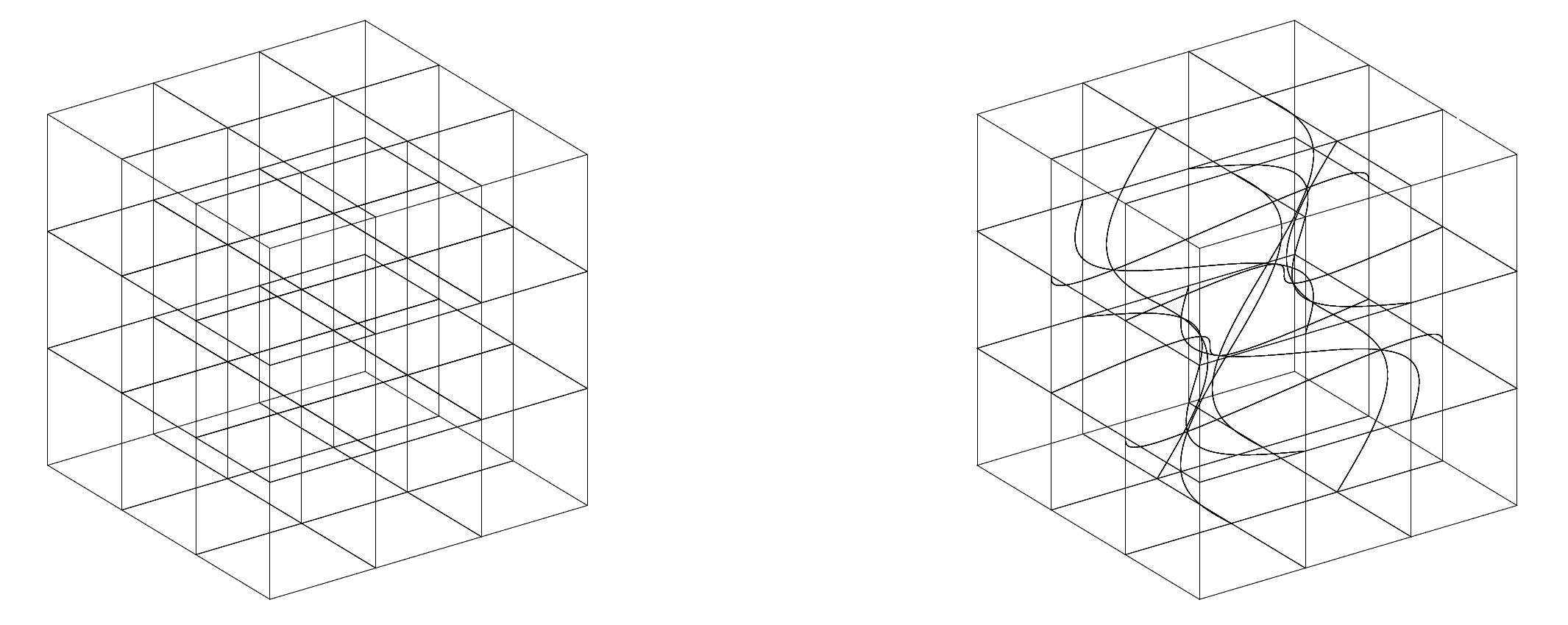
In this script, we define a mesh in a unit cube,

$\Omega = [0,1]^3.$

The mesh is of $K^3$ elements,

$\Omega_{m}=\Omega_{i+(j-1)K+(k-1)K^2}=\Omega_{i,j,k},\quad i,j,k \in\left\lbrace1,2,\cdots,K\right\rbrace.$

The mapping $\Phi_{m}=\Phi_{i,j,k}:\Omega_{\mathrm{ref}}\to \Omega_{i,j,k}$ is given as

$\Phi_{i,j,k} = \mathring{\Phi}\circ\Xi_{i,j,k},$

where $\Xi_{i,j,k}$ is a linear mapping, $\Xi_{i,j,k}:\Omega_{\mathrm{ref}}\to\left( \left[\dfrac{i-1}{K},\dfrac{i}{K}\right], \left[\dfrac{j-1}{K},\dfrac{j}{K}\right], \left[\dfrac{k-1}{K},\dfrac{k}{K}\right] \right)$ , i.e.,

$\begin{pmatrix} r\\s\\t \end{pmatrix} = \Xi_{i,j,k}(\xi,\eta,\varsigma) = \dfrac{1}{K} \begin{pmatrix} i-1 + (\xi+1)/2\\ j-1 + (\eta+1)/2\\ k-1 + (\varsigma+1)/2 \end{pmatrix},$

and $\mathring{\Phi}$ is a mapping,

$\begin{pmatrix} x\\y\\z \end{pmatrix} = \mathring{\Phi}(r,s,t) = \begin{pmatrix} r + \frac{1}{2}c \sin(2\pi r)\sin(2\pi s)\sin(2\pi t)\\ s + \frac{1}{2}c \sin(2\pi r)\sin(2\pi s)\sin(2\pi t)\\ t + \frac{1}{2}c \sin(2\pi r)\sin(2\pi s)\sin(2\pi t) \end{pmatrix},$

where $0 \leq c \leq 0.25$ is a deformation factor. When $c=0$ , $\mathring{\Phi}$ is also a linear mapping. Thus we have a uniform orthogonal mesh. When $c>0$ , the mesh is curvilinear. Two examples (left: $c=0$ , right: $c=0.25$ ) of this mesh for $K=3$ are shown below.

⭕ To access the source code, click on the [source] button at the right side or click on [crazy_mesh.py]. Dependence may exist. In case of error, check import and install required packages or download required scripts. © mathischeap.com

class crazy_mesh.CrazyMesh(c, K)[source]¶

The crazy mesh.

Parameters:

c (float) – The deformation factor, $0 \leq c \leq 0.25$ .
K (int) – The crazy mesh is of $K^3$ elements.

Example:

>>> cm = CrazyMesh(0.1, 2)
>>> e0 = cm.CT_of_element_number(0)
>>> e000 = cm.CT_of_element_index(0, 0, 0)
>>> e0 is e000
True
>>> e7 = cm.CT_of_element_number(7)
>>> e111 = cm.CT_of_element_index(1, 1, 1)
>>> e7 is e111
True
>>> e000 
<coordinate_transformation.CoordinateTransformation object at...
>>> e7 
<coordinate_transformation.CoordinateTransformation object at...

CT_of_element_index(i, j, k)[source]¶

Return a CoordinateTransformation instance for element $\Omega_{i,j,k}$ .

Note that Python index starts from $0$ . So for a CrazyMesh of $K^3$ elements, its indices, $i,j,k\in\left\lbrace 0, 1, K-1\right\rbrace$ .

Parameters:

i (int) – Element index i.
j (int) – Element index j.
k (int) – Element index k.

Returns:

A CoordinateTransformation instance.

CT_of_element_number(m)[source]¶

Return a CoordinateTransformation instance for element $\Omega_{m}$ .

Note that Python index starts from $0$ . So for a CrazyMesh of $K^3$ elements, $m\in\left\lbrace 0,1,\cdots,K^3-1\right\rbrace$ .

Parameters:: m (int) – Element No. m.
Returns:: A CoordinateTransformation instance.

class crazy_mesh.CrazyMeshGlobalBoundaryDOFs(K, N)[source]¶

We find the global numbering of the dofs on each boundary of the crazy mesh.

Parameters:

K (int) – The crazy mesh is of $K^3$ elements.
N (int) – The degree $N$ . of the to be used mimetic polynomial basis functions.

Example:

>>> K = 2
>>> N = 1
>>> B_DOFs = CrazyMeshGlobalBoundaryDOFs(K, N)
>>> FB_dofs = B_DOFs.FP
>>> FB_dofs['x_minus'] # x=0 face
array([0, 3, 6, 9])
>>> FB_dofs['x_plus'] # x=1 face
array([ 2,  5,  8, 11])
>>> FB_dofs['y_minus'] # y=0 face
array([12, 13, 18, 19])
>>> FB_dofs['y_plus'] # y=1 face
array([16, 17, 22, 23])
>>> FB_dofs['z_minus'] # z=0 face
array([24, 25, 26, 27])
>>> FB_dofs['z_plus'] # z=1 face
array([32, 33, 34, 35])

property EP¶: Find the dofs of an element in $\text{EP}_{N-1}(\Omega)$ which are on boundary of the crazy mesh of $K^3$ elements.

property FP¶

Find the dofs of an element in $\text{FP}_{N-1}(\Omega)$ which are on boundary of the crazy mesh of $K^3$ elements.

Returns:: A dict whose keys are ‘x_minus’, ‘x_plus’, ‘y_minus’, ‘y_plus’, ‘z_minus’, ‘z_plus’, and whose values are the global numbering of the dofs on the boundaries indicated by the keys.

property NP¶: Find the dofs of an element in $\text{NP}_{N}(\Omega)$ which are on boundary of the crazy mesh of $K^3$ elements.

class crazy_mesh.CrazyMeshGlobalNumbering(K, N)[source]¶

A wrapper of global numberings for discrete variables in the crazy mesh.

Parameters:

K (int) – The crazy mesh is of $K^3$ elements.
N (int) – The degree $N$ . of the to be used mimetic polynomial basis functions.

Example:

>>> K = 2
>>> N = 1
>>> GM = CrazyMeshGlobalNumbering(K, N)
>>> GM.FP
array([[ 0,  1, 12, 14, 24, 28],
       [ 1,  2, 13, 15, 25, 29],
       [ 3,  4, 14, 16, 26, 30],
       [ 4,  5, 15, 17, 27, 31],
       [ 6,  7, 18, 20, 28, 32],
       [ 7,  8, 19, 21, 29, 33],
       [ 9, 10, 20, 22, 30, 34],
       [10, 11, 21, 23, 31, 35]])
>>> GM.VP
array([[0],
       [1],
       [2],
       [3],
       [4],
       [5],
       [6],
       [7]])

property EP¶: Generate a global numbering for the dofs of an element in $\text{EP}_{N-1}(\Omega)$ on a crazy mesh of $K^3$ elements.

property FP¶: Generate a global numbering for the dofs of an element in $\text{FP}_{N-1}(\Omega)$ on a crazy mesh of $K^3$ elements.

property NP¶: Generate a global numbering for the dofs of an element in $\text{NP}_{N}(\Omega)$ on a crazy mesh of $K^3$ elements.

property VP¶: Generate a global numbering for the dofs of an element in $\text{VP}_{N-1}(\Omega)$ on a crazy mesh of $K^3$ elements.

↩️ Back to Ph.D. thesis complements (ptc).

crazy_mesh.py¶

mathischeap

Navigation

Related Topics